Surface Quasi-Geostrophic (SQG) Modeling
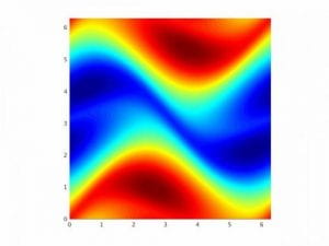
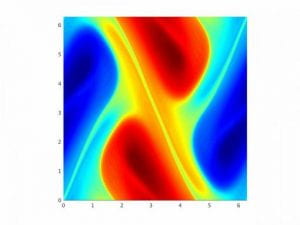
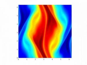
The surface quasi-geostrophic (SQG) equation is useful in modeling atmospheric phenomena such as the frontogenesis i.e., the formation of strong fronts between masses of hot and cold air. We introduce the concept of fractional spectral vanishing viscosity (fSVV) to solve conservations laws that govern the evolution of steep fronts. We apply this method to the two-dimensional surface quasi-geostrophic (SQG) equation. The classical solutions of the inviscid SQG equation can develop finite-time singularities. By applying the fSVV method, we are able to simulate these solutions with high accuracy and long-time integration with relatively low resolution.
Fractional Turbulent Flow


We purpose a fractional differential equation to govern the turbulent channel flow since the small-scale components can be described as an anomalous diffusion. The numerical results reveal that the fractional order for all different Reynolds-number has universal profile in wall unit scaling.
Fractional Cahn-Hilliard

The Cahn-Hilliard equation models the phase separation of a binary alloy at a fixed temperature. The fractional version of the Cahn-Hilliard equation arises as a gradient flow of the free energy in the negative order Sobolev space H–α, resulting in an equation that conserves mass for all positive values of α and reduces energy. A Fourier-Galerkin scheme was developed to solve the fractional Cahn-Hilliard equation. In this figure, the same random initial conditions for two different volume fractions and three different fractional orders α, and the configurations at time T = 20 are plotted. (Source: Mark Ainsworth and Zhiping Mao, “Analysis and approximation of a fractional Cahn-Hilliard equation”, SIAM J. Numer. Anal. 55 (2017), No. 4, 1689-1718.)
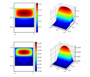
Solutions of the fractional Poisson equation, using the integral fractional Laplacian and zero Dirichlet exterior conditions, on a two-component domain corresponding to a constant right-hand-side. In the top two plots, the fractional Poisson equation is posed with the order s = 0.25, and on the bottom, it has order s = 0.75. An adaptive finite element method was developed to solve this equation. (Source: Mark Ainsworth and Christian Glusa, “Aspects of an adaptive finite element method for the fractional Laplacian: a priori and a posteriori error estimates, efficient implementation and multigrid solver”, Computer Methods in Applied Mechanics and Engineering, 327 (2017), 4-35. DOI:10.1016/j.cma.2017.08.019)

Adaptively refined grid for the fractional Poisson equation on the two-component domain, with (left) s = 0.25 and (right) s = 0.75.
Riesz spectral components

The different definitions of the fractional Laplacian lose their equivalence when they are restricted to bounded domains and boundary conditions are imposed. We numerically compared these definitions in different domains. Here, we plot the difference between the solutions of the fractional Poisson equation with the Riesz (or integral) definition and the spectral definition. The domain is L-shaped, zero Dirichlet boundary conditions are enforced, and the source term is sin(πx)sin(πy). For more comparisons, theoretical derivations and considerations for each definition, and a collection of state-of-the-art numerical approaches, see: Anna Lischke, Guofei Pang, Mamikon Gulian, Fangying Song, Christian Glusa, Xiaoning Zheng, Zhiping Mao, Wei Cai, Mark M. Meerschaert, Mark Ainsworth, and George Em Karniadakis, “What Is the Fractional Laplacian?”, arXiv preprint: 1801.09767 (2018).
More information can be found on MURI Fractional PDE site.